Making Bayesian A/B testing more accessible

Much has been written in recent years on the pitfalls of using traditional hypothesis testing with online A/B tests. A key issue is that you’re likely to end up with many false positives if you repeatedly check your results and stop as soon as you reach statistical significance. One way of dealing with this issue is by following a Bayesian approach to deciding when the experiment should be stopped. While I find the Bayesian view of statistics much more intuitive than the frequentist view, it can be quite challenging to explain Bayesian concepts to laypeople. Hence, I decided to build a new Bayesian A/B testing calculator, which aims to make these concepts clear to any user. This post discusses the general problem and existing solutions, followed by a review of the new tool and how it can be improved further.

The problem

The classic A/B testing problem is as follows. Suppose we run an experiment where we have a control group and a test group. Participants (typically website visitors) are allocated to groups randomly, and each group is presented with a different variant of the website or page (e.g., variant A is assigned to the control group and variant B is assigned to the test group). Our aim is to increase the overall number of binary successes, where success can be defined as clicking a button or opening a new account. Hence, we track the number of trials in each group together with the number of successes. For a given group, the number of successes divided by number of trials is the group’s raw success rate.

Given the results of an experiment (trials and successes for each group), there are a few questions we would typically like to answer:

1. Should we choose variant A or variant B to maximise our success rate?
2. How much would our success rate change if we chose one variant over the other?
3. Do we have enough data or should we keep experimenting?

It’s important to note some points that might be obvious, but are often overlooked. First, we run an experiment because we assume that it will help us uncover a causal link, where something about A or B is hypothesised to cause people to behave differently, thereby affecting the overall success rate. Second, we want to make a decision and choose either A or B, rather than maintain multiple variants and present the best variant depending on a participant’s features (a problem that’s addressed by contextual bandits, for example). Third, online A/B testing is different from traditional experiments in a lab, because we often have little control over the characteristics of our participants, and when, where, and how they choose to interact with our experiment. This is an important point, because it means that we may need to wait a long time until we get a representative sample of the population. In addition, the raw numbers of trials and successes can’t tell us whether the sample is representative.

Bayesian solutions

Many blog posts have been written on how to use Bayesian statistics to answer the above questions, so I won’t get into too much detail here (see the posts by David Robinson, Maciej Kula, Chris Stucchio, and Evan Miller if you need more background). The general idea is that we assume that the success rates for the control and test variants are drawn from Beta(α_A, β_A) and Beta(α_B, β_B), respectively, where Beta(α, β) is the beta distribution with shape parameters α and β (which yields values in the [0, 1] interval). As the experiment runs, we update the parameters of the distributions – each success gets added to the group’s α, and each unsuccessful trial gets added to the group’s β. It is often reasonable to assume that the prior (i.e., initial) values of α and β are the same for both variants. If we denote the prior values of the parameters with α and β, and the number of successes and trials for group x with S_x and T_x respectively, we get that the success rates are distributed according to Beta(α + S_A, β + T_A – S_A) for control and Beta(α + S_B, β + T_B – S_B) for test.

For example, if α = β = 1, T_A = 200, S_A = 120, T_B = 200, and S_B = 100, plotting the probability density functions yields the following chart (A – blue, B – red):

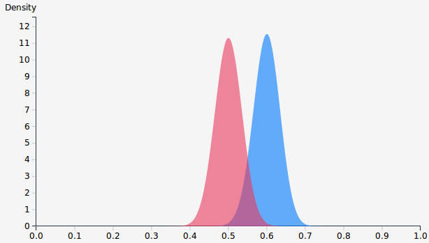
Given these distributions, we can calculate the most probable range for the success rate of each variant, and estimate the difference in success rate between the variants. These can be calculated by deriving closed formulas, or by drawing samples from each distribution. In addition, it is important to note that the distributions change as we gather more data, even if the raw success rates don’t. For example, multiplying each count by 10 to obtain T_A = 2000, S_A = 1200, T_B = 2000, and S_B = 1000 doesn’t change the success rates, but it does change the distributions – they become much narrower:

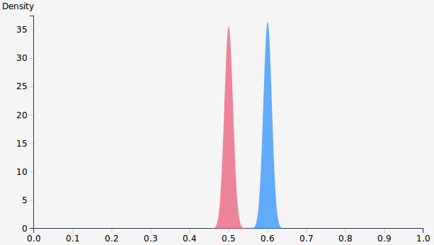
In the second case we’ve gathered ten times the data, which made the distributions much more distinct. Intuitively, this means we can now be more confident that the success rate of A is higher than that of B. Quantifying this confidence and deciding when to conclude the experiment isn’t straightforward, and should depend on factors that aren’t fully captured by the raw counts. The way I chose to address this issue is presented below, after briefly discussing existing calculators and their limitations.

Existing online calculators

The beauty of frequentist tools for significance testing is that they always give you a simple answer. For example, if we plug the numbers from the first case above (T_A = 200, S_A = 120, T_B = 200, and S_B = 100) into Evan Miller’s calculator, we get:

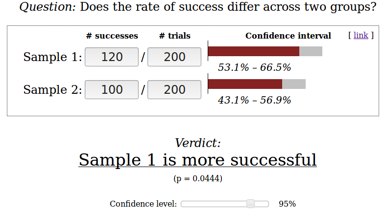
Unfortunately, both Bayesian calculators that I’m aware of have some limitations. Plugging the same numbers into the calculators by PeakConversion and Lyst would inform you that the probability of A being best is approximately 0.98, but it won’t tell you what’s the best way forward given this information. PeakConversion also outputs the 95% success rate intervals for A (between 53.1% and 66.7%) and B (between 43.1% and 56.9%), but it doesn’t let users set the prior values α and β (it uses α = β = 0.5). The ability to set priors based on what we know about our experimental setting is an important feature of Bayesian statistics that can help reduce the number of false positives. Hiding the priors in PeakConversion’s calculator makes it easier to use but less powerful than Lyst’s tool. In addition, Lyst’s calculator presents the distribution of differences between the success rates of A and B, i.e., the effect size. This is important because we may not bother implementing certain changes if the effect is negligible, even if the probability of one variant being better than the other is very close to 1.

Despite being more powerful, I find Lyst’s calculator just a bit too technical. Specifically, setting the α and β priors requires some familiarity with the beta distribution, which many people don’t have. Also, the effect size distribution is important, but can be hard to get one’s head around. Therefore, I decided to extend Lyst’s calculator, aiming to release a new tool that is both powerful and easy to use.

Building the new calculator

The source code for Lyst’s calculator is available on GitHub, so I decided to use that as the foundation of the new calculator. The first step was to convert the code from HTML, CSS, and JavaScript to Jade, Sass, and CoffeeScript, and clean up some code duplication. As the calculator is served from my GitHub Pages domain, it was easiest to put all the code in that repository. Once I had an environment and codebase that I was happy with, it was time to make functional changes:

• Change the layout to be responsive, so it’d work well on mobile devices.
• Enable sharing of results by changing the URL when the input changes.
• Provide clear instructions, so that the calculator can be used by people who don’t necessarily have a strong background in statistics.
• Allow users to set priors based on more familiar figures than the beta distribution’s α and β priors.
• Make a clear and well-justified recommendation on how to proceed.

While the first two changes were straightforward to implement, the other points were somewhat more challenging. Specifically, providing clear explanations that assume little background knowledge isn’t simple, and I still feel that the current version of the new calculator is a bit too wordy (this may be improved in the future based on user feedback – suggestions welcome). Life would be easier if everyone thought of observed values as being drawn from distributions, but in my experience this is not always the case. However, I believe it is important to communicate the reality of uncertainty, so I don’t want to hide it from users of the calculator, even at the price of more elaborate explanations.

Making the priors more intuitive was a bit tricky. At first, I thought I’d let users state their prior knowledge in terms of the mean and variance of past performance, relying on the fact that for Beta(α, β) the mean μ is α / (α + β), and the variance σ² is αβ / (α + β)²(α + β + 1). The problem is that while the mean is simple to set, as it is always in the (0, 1) range, the upper bound for the variance depends on the mean. Specifically, it can be shown that the variance is in the range (0, μ(1 – μ)). Therefore, I decided to let users quantify their uncertainty about the mean as a number u in the range (0, 1), where σ² = uμ(1 – μ). Having played with the calculator a bit, I think this makes it easier to set good informative priors. It is also worth noting that I considered allowing users to set different priors for the control and test group, but decided against it to reduce complexity. In addition, it makes sense to have the same prior for both groups – if you have a strong belief or knowledge on which one is going to perform better, you probably don’t need to run an experiment.

One of the main reasons I decided to build the calculator was because I wanted a tool that outputs a clear recommendation. This proved to be the most challenging (and interesting) part of this project, as there are quite a few options for Bayesian stopping rules. After reading David Robinson’s review of the limitations of a stopping rule based on the expected loss, and a few of the other resources mentioned in his post, I decided to go with a combination of the third and fourth rules tested by John Kruschke. These rules rely on a threshold of caring, which is the minimum effect size that is seen as significant by the user. For example, if we’re running experiments on the conversion rate of a landing page, we may decide that we don’t care if the absolute change in conversion rate is less than 0.1%. Given this threshold and data from the experiment, the following recommendations are possible:

1. Stop the experiment and implement either variant, because the difference between the variants is smaller than the threshold.
2. Stop the experiment and implement the winning variant, because the difference between the variants is greater than the threshold.
3. Keep running the experiment, because there isn’t enough data to make a decision.

Formally, Kruschke’s rules work as follows. Given the minimum effect threshold t, we define a region of practical equivalence (ROPE) to zero difference as the interval [-t, t]. Then, we compare the ROPE to the 95% high density interval (HDI) of the distribution of differences between A and B. When comparing the ROPE and HDI, there are three options that correspond to the recommendations above:

1. The ROPE is completely contained in the HDI (stop the experiment and implement either variant).
2. The intersection between the ROPE and HDI is empty (stop the experiment and implement the winning variant).
3. The ROPE and HDI only partly overlap (keep running the experiment).

Kruschke’s post shows that making the rule more restrictive by adding a notion of user-settable precision can reduce the rate of false positives. The idea is to stop only if the HDI is narrower than precision multiplied by the width of the ROPE. Intuitively, this forces the experimenter to collect more data because it makes the posterior distributions narrower (as shown by the charts above). I found it hard to explain the idea of precision, and didn’t want to confuse users by adding another parameter, so I decided to use a constant precision value of 0.8. If the ROPE and HDI don’t overlap, the tool makes a recommendation to stop, accompanied by a binary level of confidence: high if the precision condition is met, and low otherwise.

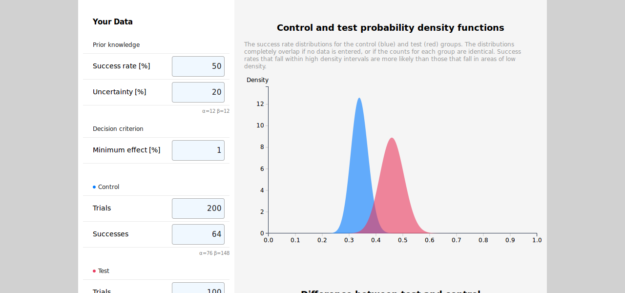
Putting in the numbers from the running example (T_A = 200, S_A = 120, T_B = 200, and S_B = 100) together with a minimum effect of 1%, prior success rate of 50%, and 57.74% uncertainty (equivalent to α = β = 1), we get the following output:

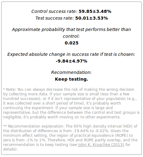
The full results also include plots of the distributions and their high density intervals. I’m pretty happy with the richer information provided by the calculator, though it still has some limitations and areas that can be improved.

Limitations and potential improvements

As mentioned above, I’d love to reduce the wordiness of the calculator while keeping it self-contained, but I need some feedback to understand if any explanations are redundant. It’d also be great to reduce the reliance on magic numbers, such as the 95% HDI and 0.8 precision used for generating a recommendation. However, making these settable by users would increase the complexity of using the calculator, which is already harder to use than the frequentist alternative. Nonetheless, it’s important to remember that oversimplification is the reason why it’s easier to make the wrong decision when following the classical approach.

Other potential changes include switching to a closed-form formula rather than draws from a distribution, comparing more than two variants, and improving Kruschke’s stopping rules by simulating more scenarios than those considered in his post. In addition, I’d like to go beyond binary responses (success/failure) to support continuous rewards (e.g., revenue), and allow users to specify different costs for the variants (e.g., implementing B may cost more than sticking with A).

Finally, it is important to keep in mind that significance testing can’t tell you whether your sample is representative of the population. For example, if you run an experiment on a very popular website, you can get a sample of thousands of people within a few minutes. Concluding an experiment based on such a sample is probably a bad idea, as it is plausible that you would reach different conclusions if you kept running the experiment for a few days, to reduce the effect that the time of day has on the results. Similarly, a few days may not be enough if your user population behaves differently on weekends – you would need to run the experiment over a few weeks. This can be extended to months and years to rule out seasonal effects, but it is up to the experimenter to weigh the practicality of considering such factors versus the need to make decisions (see articles by Peep Laja, Martin Goodson, Sam Ju, and Kohavi et al. for more details). The main thing to remember is that you just cannot completely eliminate uncertainty and the need to consider background knowledge, which is why I believe that helping more people follow the Bayesian approach is a step in the right direction.