Many is not enough: Counting simulations to bootstrap the right way

Previously, I encouraged readers to test different approaches to bootstrapped confidence interval (CI) estimation. Such testing can done by relying on the definition of CIs: Given an infinite number of independent samples from the same population, we expect a ci_level CI to contain the population parameter in exactly ci_level percent of the samples. Therefore, we run “many” simulations (num_simulations), where each simulation generates a random sample from the same population and runs the CI algorithm on the sample. We then look at the observed CI level (i.e., the percentage of CIs that contain the true population parameter), and say that the CI algorithm works as expected if the observed CI level is “not too far” from the requested ci_level.

Keen observers may notice that the language I used to describe the process isn’t accurate enough. How many is “many” simulations? How far is “not too far”?

I made a mistake by not asking and answering these questions before. I decided that num_simulations=1,000 is a reasonable number of simulations, and didn’t consider how this affects the observed CI level. The decision to use num_simulations=1,000 was informed by practical concerns (i.e., wanting the simulations to finish within a reasonable timeframe), while ranges for the observed CI level were determined empirically – by observing the results of the simulations rather than by considering the properties of the problem.

The idea of using simulations to test bootstrapped CIs came from Tim Hesterberg’s What Teachers Should Know about the Bootstrap. The experiments presented in that paper used num_simulations=10,000, but it wasn’t made clear why this number was chosen. This may have been due to space limitations or because this point is obvious to experienced statisticians. Embarrassingly, my approach of using fewer simulations without considering how they affect the observed CIs can be seen as a form of Belief in The Law of Small Numbers.

Fortunately, it’s not hard to move away from belief in the law of small numbers in this case: We can see a set of simulations as sampling from Binomial(n=num_simulations, p=ci_level), where the number of “successes” is the number of simulations where the true population parameter falls in the CI returned by the CI algorithm. We can define our desired level of confidence in the simulation results as the simulation confidence, and use the simulation confidence interval of the binomial distribution to decide on a likely range for the observed CI level.

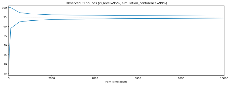
To make this more concrete, here’s a Python function that gives the observed CI level bounds for different values of num_simulations, given the ci_level and simulation confidence. The output from running this function with the default arguments is plotted below.

import numpy as np
import pandas as pd
import scipy.stats
 
def get_observed_ci_bounds(
        all_num_simulations=(10, 100, 500, 1000, 2000, 5000, 10000),
        ci_level=0.95,
        simulation_confidence=0.99
    ):
    return pd.DataFrame(
        index=pd.Series(all_num_simulations, name='num_simulations'),
        data=[
            np.array(
                scipy.stats.binom.interval(simulation_confidence,
                                           n=num_simulations,
                                           p=ci_level)
            ) / num_simulations
            for num_simulations in all_num_simulations
        ],
        columns=['low', 'high']
    ) * 100
 
 
>>> print(get_observed_ci_bounds())
num_simulations    low    high
10               70.00  100.00
100              89.00  100.00
500              92.40   97.40
1000             93.10   96.70
2000             93.70   96.20
5000             94.18   95.78
10000            94.43   95.55

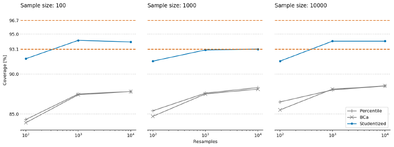
Therefore, when setting num_simulations to 1,000 (as I did in the experiments I presented previously), we can be 99% confident that the observed CI level of a perfect CI algorithm would be between 93.1% and 96.7% when asked to generate 95% CIs. As shown by the following figure, this doesn’t materially change my previous conclusions: On the dataset from those experiments, the Studentized algorithm delivers satisfactory results, while the Percentile and BCa algorithms are quite far from perfection. And of course, we can now quantify their distance from perfection – the CIs they yield in the best case would be acceptable if we wanted 90% CIs, where we expect the observed CI to be in the 87.5% to 92.4% range (obtained by running the function above with ci_level=0.9). As there are better alternatives, I believe that this is a good enough reason to avoid using the Percentile and BCa algorithms.

Notes: See this notebook for code – use the same environment as the original notebook. The cover photo is by Dima D from Pexels.